Data & Exploratory Analysis

The SLICE-3D dataset, the class imbalance, and the exploratory figures

The problem

The task is automated triage of skin-lesion crops extracted from 3D total-body photography (TBP): each crop must be classified as malignant or benign so that high-risk lesions are flagged for clinical review. The clinical objective is high sensitivity — catching nearly every malignancy — at an acceptable false-positive rate.

The dataset

ISIC-2024 SLICE-3D is a corpus of lesion crops from TBP, which images every visible mole on a patient in a single capture. Each row is one lesion: a small square JPEG crop plus a tabular record of measurements computed by the TBP vendor’s software (geometry, color, 3D position) and clinical context (age, sex, body site).

Fact	Value
Lesion crops (rows)	401,059
Malignant lesions	393
Benign lesions	400,666
Prevalence	0.098% — about 1 malignant per 1,021 crops
Unique patients	1,042
Patients with ≥1 malignant lesion	259 (24.9%)
Columns	55 (35 float, 18 string, 2 int)
Real (non-leak) feature columns	36
Imaging	every crop is a TBP tile (`TBP tile: close-up`); 2 subtypes (`3D: XP`, `3D: white`)
Source institutions	7 (MSKCC, Hospital Clínic Barcelona, Univ. Basel, Frazer Institute/UQ, ACEMID MIA, MedUni Vienna, Univ. Athens)

Data are patient-grouped: a patient contributes many correlated lesions, so the unit of independence is the patient, not the crop.

Representative crops

Figure 1: Five malignant (top) and five benign (bottom) crops, annotated with clinical longest diameter. Malignant lesions trend larger, more color-heterogeneous, and more border-irregular; benign nevi are smaller and more uniform.

The challenge

Extreme class imbalance. At 0.098% prevalence, a constant “benign” predictor is 99.9% accurate and clinically useless. With only 393 positives, fold variance and leakage dominate model choice.
The official metric. Scoring uses partial AUC above 80% TPR (pAUC@80), the area under the ROC restricted to the high-sensitivity tail — see Methods → The metric. Accuracy and plain AUC are unsuitable.
No external, no synthetic. Only SLICE-3D is permitted; no external dermoscopy archives and no generative/synthetic positives. ImageNet-pretrained weights are allowed; external training data is not.
Efficiency is a first-class axis. Every reported model logs parameters, FLOPs, and single-thread CPU latency alongside pAUC; a model is retained only if it earns its cost.

Image details

The crops are variable-size square JPEGs, 61–239 px on a side (median/mean ≈ 131/133 px), ~2.8 KB each. Two consequences for the image experts:

128 px ≈ native median. Training at 128 px is near the crops’ natural resolution; epochs are cheap and no detail is discarded.
224 px upsamples. The 224 px model receives the same lesion interpolated larger, not extra pixels. The measured 224 px gain (0.15311 → 0.15821) is therefore a capacity / training-dynamics effect (larger receptive field, more effective augmentation), not added image detail. Resolution is treated as a frontier axis, so both points are retained.

Missingness

Three real feature columns have missing values; all others are complete.

Column	Missing
`sex`	2.87%
`anatom_site_general`	1.44%
`age_approx`	0.70%

Train-only leak columns (dropped)

Several columns exist only in the training split and encode the answer or post-biopsy pathology. They are used for EDA framing only and dropped before training:

iddx_full, iddx_1 … iddx_5 (iddx_1 is Benign / Malignant / Indeterminate), mel_mitotic_index, mel_thick_mm, lesion_id, and tbp_lv_dnn_lesion_confidence (a vendor model’s confidence — unavailable at inference and effectively a label proxy).

Exploratory figures

All figures are generated by reports/eda/make_eda.py (read-only on data/, SEED = 42, Okabe-Ito colorblind-safe palette).

Fig 1 — Class imbalance & fold stratification

Figure 2: Class imbalance and per-fold positive counts.

400,666 benign vs 393 malignant (0.098% prevalence). The five patient-grouped CV folds each hold 77–83 positives (~0.096–0.103% prevalence per fold); stratification is tight and no fold is starved of signal, a precondition for trustworthy OOF estimates.

Fig 2 — Patient structure

Figure 3: Per-patient lesion counts; malignant-carrying patients hold most of the data.

1,042 patients with a heavily right-skewed lesion count (median 241, max 9,184). The 259 patients carrying at least one malignant lesion hold 39% of all crops. Because a patient’s lesions are correlated, splits must be patient-grouped: any patient straddling folds leaks information.

Fig 3 — Demographics

Figure 4: Age, sex, and body-site malignant rates.

Malignant lesions skew older (peak ~60–75), males contribute most crops, and head/neck stands out:

Body site	n	Malignant rate
head/neck	12,046	0.648%
anterior torso	87,770	0.093%
posterior torso	121,902	0.084%
upper extremity	70,557	0.081%
lower extremity	103,028	0.071%

Head/neck carries ~7× the baseline malignant rate of any other site despite being the smallest site — a strong site prior.

Fig 4 — Lesion size

Figure 5: Clinical diameter and TBP area: malignant ~2× larger.

On both clinical longest diameter and TBP area, the malignant distribution is shifted ~2× larger than benign. Raw lesion size is a strong, cheap univariate signal; its patient-relative version is stronger (see Ablations).

Fig 5 — Color & border signals

Figure 6: Hue, contrast, border/color irregularity, eccentricity.

Hue angle (tbp_lv_H) separates the classes most cleanly — univariate AUC 0.81 on a single feature. Lesion-skin contrast, border/color irregularity, and eccentricity shift toward higher values for malignant lesions, indicating independent color/geometry signal.

Fig 6 — Correlation of key TBP features

Figure 7: Correlation heatmap of 21 core geometry/color features.

The core features form tight blocks (a size group: diameter / area / perimeter / minor-axis; a color group: A / B / ΔA / ΔB). The GBDT therefore sees substantial redundancy; a small number of axes capture most of the variance.

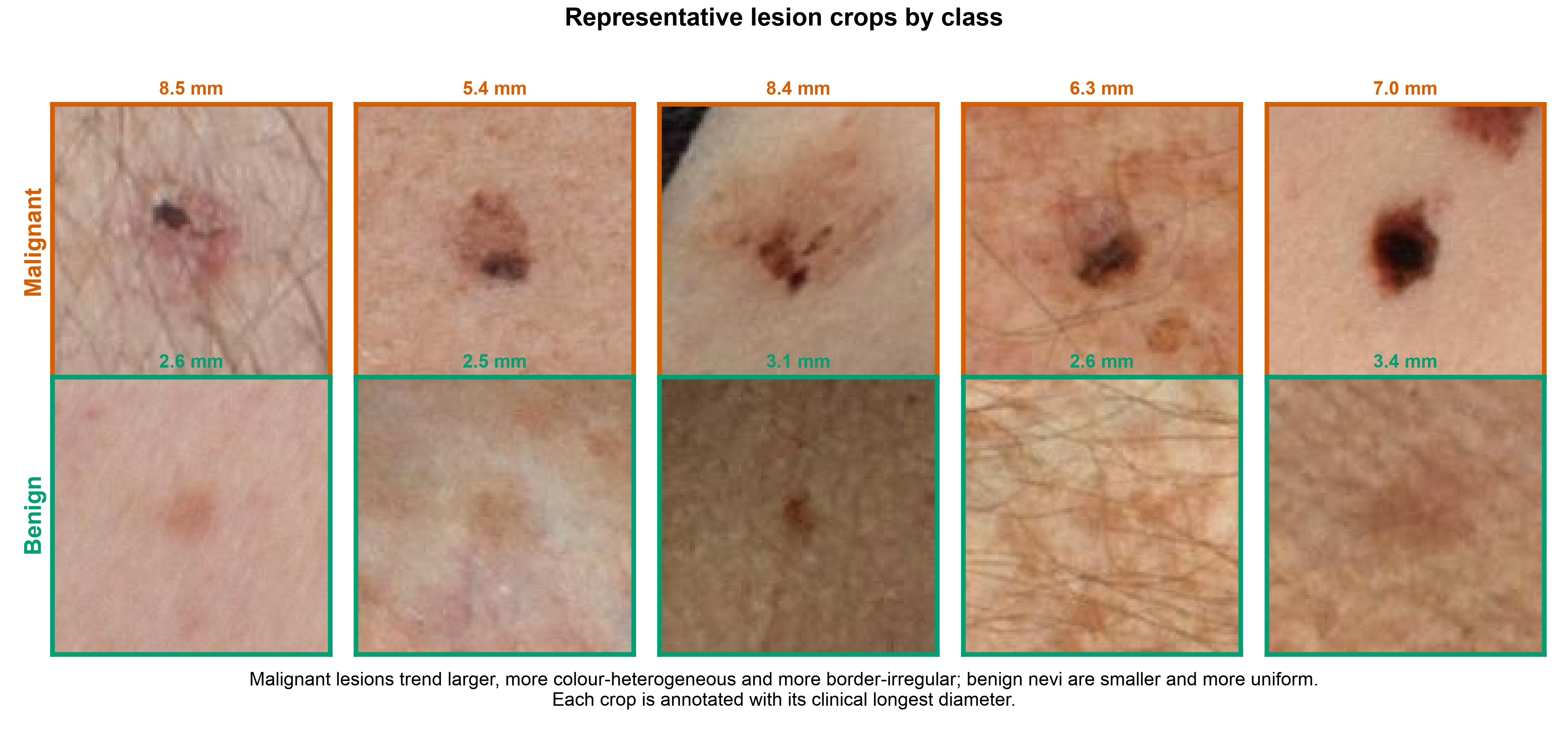
Fig 7 — Sample lesion crops

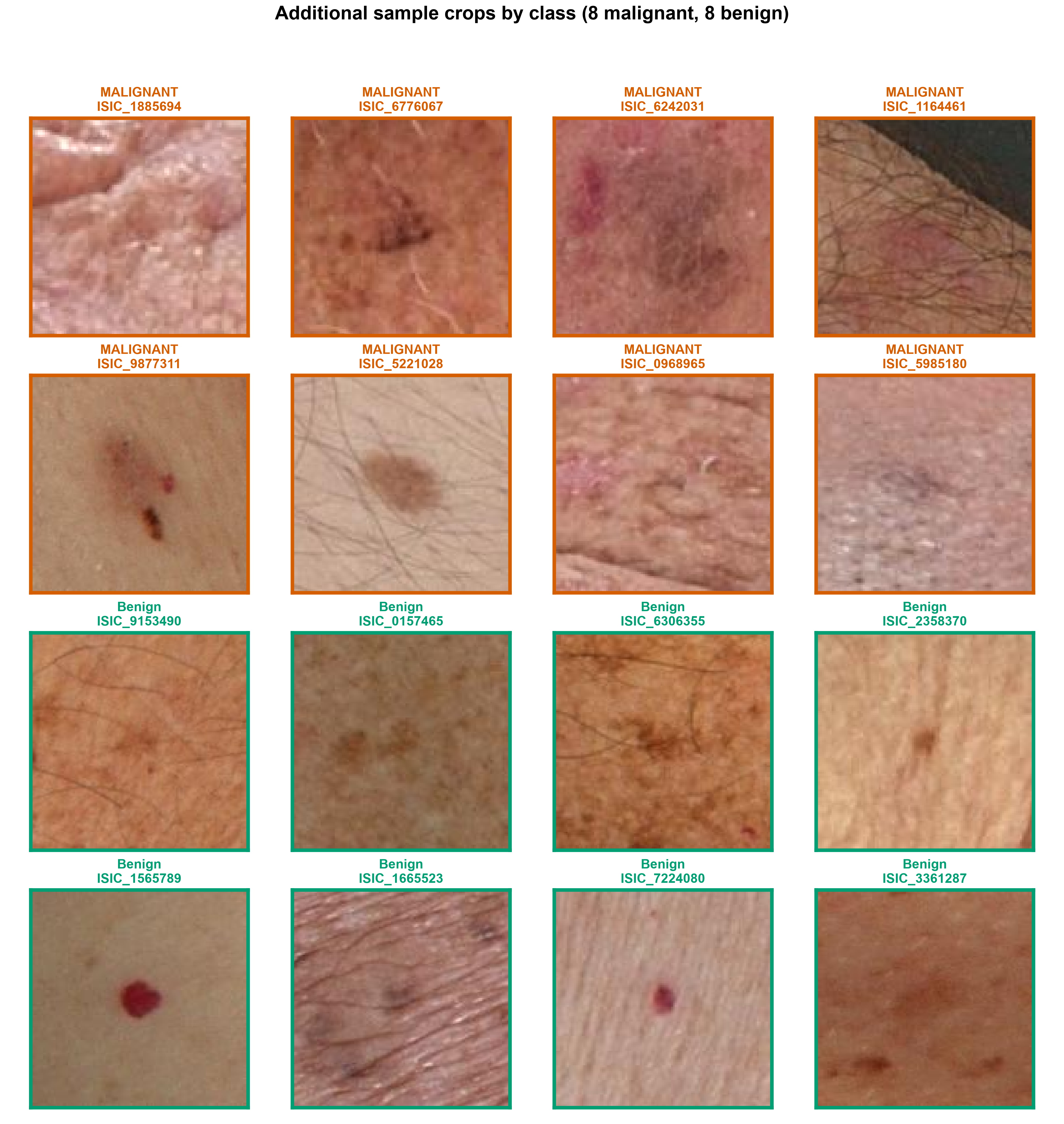
Figure 8: Eight malignant (top) vs eight benign (bottom) crops.

Malignant lesions tend to be larger, darker, and more color-varied, but visual overlap with benign is large. The overlap motivates a learned image expert on top of the tabular features and explains why the image expert alone (0.15821) does not exceed the tabular expert (0.16890).

Fig 8 — Image-embedding class separation

Figure 9: PCA-50 → t-SNE of ConvNeXtV2-nano OOF embeddings.

A t-SNE of the small CNN’s OOF embeddings (all 393 positives + 3,000 random negatives): the malignant points concentrate into a recognizable region of feature space. A small CNN learns a malignancy-relevant representation, supporting the use of its OOF probability as a stacked GBDT feature.

Fig 9 — Ugly-duckling illustration

Figure 10: Three patients: the malignant lesion sits at the top of its own size distribution.

For three patients with one malignant lesion among many benign ones, the malignant lesion sits at the top of its own patient’s size distribution (98th–100th percentile) — the concrete basis for the within-patient deviation features.

The ugly-duckling sign, quantified

392 of 393 malignant lesions belong to a patient who also has benign lesions, so almost every positive can be judged against that patient’s own normal moles.
On clin_size_long_diam_mm, the malignant lesion sits at a median 88th within-patient percentile; 45.7% of malignant lesions fall in the top 10% of their own patient’s lesion sizes.

This is the quantitative basis for the engineered patient-relative features.

Summary of findings

Imbalance defines the task. 0.098% prevalence motivates partial-AUC-above-80%-TPR scoring and mandatory patient-grouped, target-stratified CV. The folds hold 77–83 positives each with no patient straddling folds.
Tabular signal is strong and cheap. Hue tbp_lv_H reaches univariate AUC 0.81, and lesion size shows a clean ~2× malignant shift — the evidence base for the LightGBM-first architecture.
The ugly-duckling sign is quantitatively present and is the dominant signal in the trained model (~65% of GBDT gain; see Results).
The small CNN adds an orthogonal axis. Its embeddings cluster the positives despite heavy visual overlap in raw crops, justifying a stacked image OOF probability; head/neck’s ~7× elevated rate provides a site prior.

Continue to Methods →